 Age-structural modelling
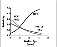
In the statistical analysis shown below (Table 1), the logistic regression model employs the country-level median age as the only continuous independent variable. In these “age-structural analyses”, logistic regression has been used to determine (1.) whether, or not, the presence of a specific, discrete condition (the dependent variable; 0 or 1) varies as states advance across the age-structural transition. If, indeed, it varies across this transition, then (2.) age-structural methods proceed to determine how that specific condition varies (its functional form); and (3.) the level of certainty that is associated with that variation (its confidence interval).
In age-structural models, the dependent variable (composed of data coded “1” or “0”) must be discrete, or discretized by creating a gradient of discrete categories. Examples of discrete conditions include the presence or absence (in a year) of a type of political regime, such as a liberal democracy (shown in Table 1), or the presence or absence of an intra-state conflict. Examples of discretized variable include the attainment of specific levels of per-capita income (e.g., the World Bank’s Upper-middle Income Category), or levels of educational attainment (secondary school participation).
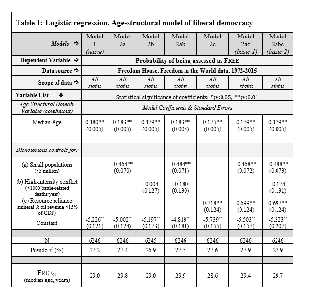
Table 1. Logistic regression statistical table for the age-structural model of liberal democracy. Dichotomous controls are small populations, the presence of high-intensity conflict, and reliance on oil or mineral resources (each defined in the table).
Control Variables
In my own experience, I have found it useful to begin with the simplest form of the age-structural model—the naïve model, which is devoid of any control variables (Model 1, example in Table 1). To refine this model, I have added dichotomous (presence or absence) control variables, or combinations of these three variables, to refine the naïve model. States with these qualities often, but not always, perform differently than the larger group of states. Before graphing the function, running experiments with other dichotomous variables, or identifying exceptional states, I typically find it useful to control for these three factors, depending on the dependent variable:
(a.) States with small populations. This factor identifies states with a mid-year population of fewer than 5.00 million. The source of this estimate was the UN Population Division’s 2015 revision of World Population Prospects (UNPD, 2015).
(b.) States engaged in high intensity conflict. A state is deemed to be in high intensity conflict if, for that year, it experiences more than 1000 battle-related deaths, according to the current version of the UCDP Conflict Dataset (Uppsala Conflict Data Project and Peace Research Institute, Oslo [UCDP/PRIO], 2014; Gleditsch et al., 2002).
(c.) Resource-reliant states. A state was deemed as experiencing significant oil and mineral wealth if revenues from these resources comprised over 15.0 percent of GDP. Annual levels of oil revenue, mineral revenue and GDP were obtained from the 2015 version of the World Bank’s World Development Indicators (World Bank Group [WB], 2015).
Thus, current analyses typically feature controlled models (Model 2, examples in Table 1) that feature various combinations of this model (e.g., Models 2a, 2ab, 2ac, 2bc, 2abc). As a general observation, the effect of small population (a) generally produces the strongest statistical impact on a naïve model. The control for high intensity conflict (b) has occasionally been statistically significant, particularly in health and income-related models, but is omitted when the dependent variable is a conflict-related variable. Oil-mineral reliance (c) has been statistically significant in most age-structural models.