Age-structural functions: their directionality and punctuality

What is an Age-structural Function?

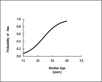
    An age-structural function is a two-dimensional graphic form of an age-structural model. This function describes a range (Y-axis) of probabilities of being within a category at all points (median ages) across the age-structural domain (the X-axis of the graph). To neatly capture nearly all recent positions in the age-structural transition, now and in the foreseeable future, the standard form of this graph extends over a domain that begins at a median age of 15 years and ends at 55 years. This standardized form is not perfect. Over the course of UN Population Division (UNPD) estimates (1950 to 2015), the populations of a few states (including Niger in 2015) have experienced median ages below 15.0 years. On the high side of the domain, however, no country-level age structure has yet gone beyond a median age of 48. Nonetheless, the UN Population Division projects that Japan will reach a median age higher than 50 years before 2030, and that several European and additional East Asian countries will follow it into the post-mature phase (a median age of 45.6 or higher) soon thereafter.

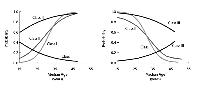
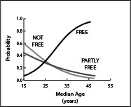
Not all age-structural functions that are fit to data by an age-structural model are qualitatively similar. Age-structural functions have been categorized into three qualitative classes (I, II, III), according to the conditions associated with the age-structural function that they describe (Fig. 1). These conditions influence the form and fit of the age-structural function.[i]

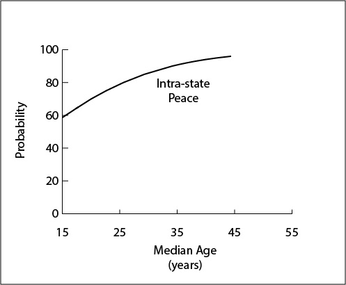
These three classes suggest differences in the strength of the relationship’s directionality and punctuality. Functional directionality can also be expressed as the ratio between the frequency at which it advances into a category, relative to the frequency at which it retreats back into this category. Class I age-structural functions (such as income and education functions) express high ratios of directionality and feedback between the indicator and movement along the age structural transition (or fertility decline). Class III functions (such as the frequency of intra-state conflict or the initiation of intra-state conflict) typically express low ratios. Class II functions (such as being assessed as Free in Freedom House’s annual survey) are like class I functions, but not as directional. States backslide more often, and there may be very little feedback, if any, associated with the relationship. Functional punctuality measures the tendency for advancement to be associated with a particular median age. This quality can be measured by the steepness of the curve (i.e., value of first derivative) at its inflection point (where p=0.50). Class I age-structural functions are most punctual; class III, the least.


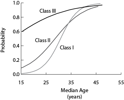
Figure 1. Three classes of age-structural function (I, II, III). Each is associated with a particular set of dynamics exhibited by states, in terms of a categorical dependent variable (Y), over the length of the age-structural domain (X axis).


[i] Cincotta, R. 2017. “The Age-structural Theory of State Behavior.” in Oxford Reference Encyclopedia: Empirical International Relations Theory, edited by W. Thompson. Oxford: Oxford University Press. Download here.

Three Classes of Age-structural Functions

Age-structural Functions: Classes I, II, and III

A Class I Function: The World Bank’s Income Categories.

The World Bank Income Category Model (ASM-GNI) is composed of four class I age-structural functions that generate expectations of the age-structural timing of each of the World Bank’s standard income categories (Fig. 1). These categories are based on gross national income per capita (GNI per capita), calculated in current-year (or other standard year) US dollars using the World Bank’s Atlas Method (WB, 2016). States rarely slip from a higher to lower category.

Figure 1. Examples of Class I age-structural functions: the World Bank’s Income Categories. Class I functions depict the state’s attainment of a discrete level that is irreversible or nearly so. 

GNI per capita (Atlas Method) data were transformed into four dependent variable data sets, each composed of presence of absence data (0,1). For the World Bank’s Low Income Category was transformed to indicate whether it was in the category (1), or not (0).  For the following three higher categories (Lower-middle Income, Upper-middle Income, and High Income), GNI per capita data were transformed to identify whether the state was in the chosen category or a higher category (1), or in a lower category (0).

The functions displayed in this graph are the product of Model 2ac, which uses two statistically significant controls (p<0.05): small population size (<5.0 million), and reliance on oil or mineral resources (>15.0 percent of GDP). Thus controlled, relatively narrow 0.95 confidence intervals, reaching a maximum of +0.9 years on the median age axis at low median ages, surrounds each of the logistic functions.

While still untested by forecasting and experimentation, or examined in terms of the behavior of its exceptional states, the model reveals fresh aspects of the relationship between age structure and income. While it appears that states routinely achieve the World Bank’s Lower-middle Income category in the youthful phase of the age-structural transition (median age, <25 years), the results of modeling suggest that states must be well into the intermediate phase of the age-structural transition (thus attain fertility levels below 2.5 children per woman) to attain Upper-middle Income status—a milestone on the pathway to economic development at which development donors graduate countries from basic sectors of development.

Notably, the demographic window of opportunity—introduced by UNPD (2004) to estimate the period of greatest potential for economic development—coincides closely with the period when most states attain Upper-middle Income status. In its original formulation, the demographic window was calculated open when proportions of children, 0 to 14 years of age dipped below 30 percent of the total population, and seniors, 65 years and older, remained below 15 percent of the population. In the age-structural domain, that ranges from a median age of about 26 years to about 41 years.


A Class II Function: The Presence of Liberal Democracy.

The age-structural model of liberal democracy (ASM-LD) generates timed expectations of the likelihood of being assessed at a high level of democracy across the age-structural axis (Fig. 2). The ASM-LD is the most well-studied of all age-structural functions, having been investigated by three independent research efforts, each using different measures of age structure (several variations of “youth bulge” measures, median age), and various indicators of democracy. Indications of democracy include Freedom House’s Free status (Cincotta 2008, 2008-09), high levels (8 to 10) of Polity IV regime scores (Cincotta & Doces, 2012; Weber, 2012), and high levels of voting as a proportion of eligible voters (Dyson, 2013). The conclusions were similar. Moreover, the ASM-LD is the subject of several successful forecasts and statistical experiments, which in turn have inspired additional hypotheses and modeling (Cincotta, 2008-09; Cincotta & Doces, 2012; Cincotta, 2015a, 2015b).

Figure 2. An example of a Class II function: the age-structural function depicting the probability of being assessed as FREE in Freedom House’s annual survey.

The functional form of the ASM-LD, shown here (Fig. 2), plots the timed expectation of attaining Free in Freedom House’s annual survey (Model 2ac, Table 1), as a probability calculated across the age-structural domain (Cincotta, 2015b). The most rapid pace of shifts to Free from lower categories should be expected to occur around the theoretical infliction point, where the probability of being assessed as Free is 0.50. This point, called Free50, is at about 29.5 (+0.5) years of median age.

A Class III Function: The Presence of Intra-state Peace.

The Age-structural Model of Intra-state Peace (ASM-ISP) predicts the probability of the absence of intra-state conflict across the age-structural domain (Fig. 3). The model draws its data on the presence or absence of intra-state conflict (>25 battle-related deaths per year) from the UCDP-PRIO Conflict Database, maintained and published cooperatively by the Uppsala Conflict Database Project (UCDP) and Peace Research Institute of Oslo (PRIO) (UCDP/PRIO, 2016; Gleiditsch et al., 2002; Themnér & Wallensteen, 2013). Its function (Fig. 3) is a class III age-structural function, based upon the ASM-ISP, with controls for small population (<5.0 million), and natural resource reliance (resource rents <15.0 percent of GDP).

Figure 3. An example of a Class III function: the age-structural function of intra-state peace (absence of an intra-state conflict).

The ASM-ISP is neither a tightly fit nor strongly predictive model—its gradual slope is not conducive to forecasting. It is nonetheless useful in mapping states, now and over the next two decades, that are generally vulnerable to the outbreak of intra-state conflict and other forms of political violence. It is worth noting that, according to the ASM-IP, at a median age of 15.0 years, roughly 60 percent of all states are unlikely to be experiencing an intra-state conflict.  Further investigations of the function indicate that while civil conflicts appear almost exclusively in the youthful portion of the age-structural domain (median age of 25 years or less), ethnoreligious conflicts extend throughout the domain (see Yair, 2016).

Attachments

Age-structural Models

Age-structural Models: the Idea


The age-structural domain is the unifying feature of Age Structural Theory. Rather than consider relationships over chronological time, age-structural models re-position state behaviors on the age-structural domain—an X-axis that follows the continuous path of the age-structural transition, situating it as the principal independent variable. The age-structural domain, measured in median age, is the only continuous independent variable in logistic regression analysis. All controls and treatment variables are dichotomous (0,1). Likewise, the functional forms that are fitted to data by logistic regression are displayed across a domain beginning at a median age of 15 years and ending at 55 years.

Each age-structural model begins as a hypothesis, whether generated notionally (from theory) or observationally, that a measurable state behavior is typically associated with the movement of states through the age-structural transition. It is important to stress—and periodically re-iterate—that these models begin as a hypothesis that is epistemologically situated at the very edge of Age-structural Theory. Some age-structural models have been strengthened and brought into the more certain body of theory by repeated in-sample testing, out-of-sample testing, and some form of successful prediction. A few others—particularly hypotheses associated with the age-structural model of liberal democracy (ASM-LD)—have demonstrated their utility by out-competing other methods of analysis and by exposing original insights into the processes under study.

In my analyses, age-structural models employ the country-level median age as the only continuous independent variable. In these analyses, logistic regression has been used to determine (1.) whether, or not, the presence of a specific, discrete condition (the dependent variable) varies as states advance across the age-structural transition. If, indeed, it varies across this transition, then (2.) age-structural methods proceed to determine how that specific condition varies (its functional form); and (3.) the level of certainty that is associated with that variation (its confidence interval).

In age-structural models, the dependent variable (composed of data coded “1” or “0”) must be discrete, or discretized by creating a gradient of discrete categories. Examples of discrete conditions include the presence or absence (in a year) of a type of political regime, or the presence or absence of an intra-state conflict. Examples of discretized variable include the attainment of specific levels of per-capita income (e.g., the World Bank’s Upper-middle Income Category), or levels of educational attainment (secondary school participation).

For logistic regression to produce a reasonable fit to these data, the frequency of the dependent variable, as it is sampled across the age-structural domain, must be adequately described by a logistic function—a monotonic sigmoid curve generated by the Verhulst equation (an S-shaped function, beginning low and approaching an upper asymptote), or to some segment of a logistic curve (Maynard, 2001). Therefore, a segment of a logistic function can neither be fit adequately to frequency data that (a.) rises substantially and then falls, nor (b.) falls substantially and then rises again across the domain.

Age-structural Theory is a reductionist project. Operating on a single, continuous X-axis simplifies statistical analyses and permits the visual display of relationships on a two-dimensional graph. And, like all simplified statistical theories, it has limitations. Firstly, it suffers from the “small number problem”—predictions are most successful when considering clusters of states, rather than betting on a single state. Secondly, by itself, taking only median age into account, age-structural models are blind to the influence of non-demographic and sub-national demographic factors. Unless these are noted through observation, studied through separate analyses, or added experimentally as discrete (0,1) variables to the statistical analysis, its reliance on the country-level scalar measure of median age as the lone continuous domain of its analysis can obscure important factors. For example, observations of the functional form of the age-structural model of liberal democracy have shown that presence of a small population size (under 5 million) and regime types have substantial impact on outcomes (Cincotta, 2015a, 2015b; Weber, 2013).

In its classic form (which was used to describe constrained population growth), the logistic function begins at its lowest point, accelerates to an inflection point, decelerates, and then levels off as it approaches an upper asymptote. However, this function can also be parameterized to operate in reverse: to begin at its high point and descend to a lower asymptote. Upward or downward sections of the function can be fit to data, as well.