Three Classes of Age-structural Functions

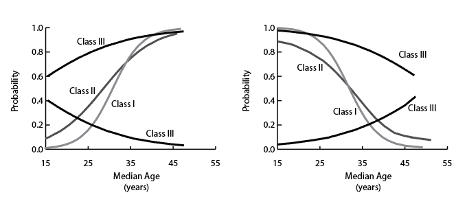
Age-structural Functions: Classes I, II, and III

A Class I Function: The World Bank’s Income Categories.

The World Bank Income Category Model (ASM-GNI) is composed of four class I age-structural functions that generate expectations of the age-structural timing of each of the World Bank’s standard income categories (Fig. 1). These categories are based on gross national income per capita (GNI per capita), calculated in current-year (or other standard year) US dollars using the World Bank’s Atlas Method (WB, 2016). States rarely slip from a higher to lower category.

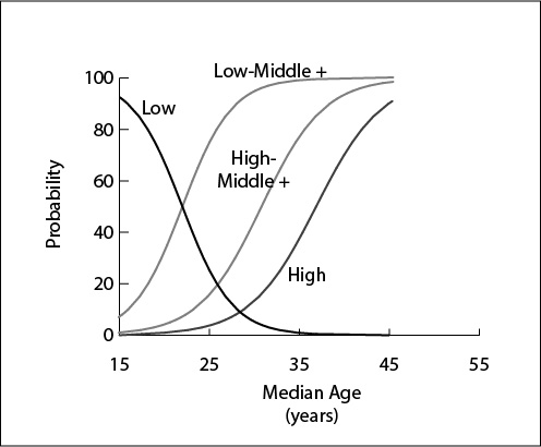
Figure 1. Examples of Class I age-structural functions: the World Bank’s Income Categories. Class I functions depict the state’s attainment of a discrete level that is irreversible or nearly so. 

GNI per capita (Atlas Method) data were transformed into four dependent variable data sets, each composed of presence of absence data (0,1). For the World Bank’s Low Income Category was transformed to indicate whether it was in the category (1), or not (0).  For the following three higher categories (Lower-middle Income, Upper-middle Income, and High Income), GNI per capita data were transformed to identify whether the state was in the chosen category or a higher category (1), or in a lower category (0).

The functions displayed in this graph are the product of Model 2ac, which uses two statistically significant controls (p<0.05): small population size (<5.0 million), and reliance on oil or mineral resources (>15.0 percent of GDP). Thus controlled, relatively narrow 0.95 confidence intervals, reaching a maximum of +0.9 years on the median age axis at low median ages, surrounds each of the logistic functions.

While still untested by forecasting and experimentation, or examined in terms of the behavior of its exceptional states, the model reveals fresh aspects of the relationship between age structure and income. While it appears that states routinely achieve the World Bank’s Lower-middle Income category in the youthful phase of the age-structural transition (median age, <25 years), the results of modeling suggest that states must be well into the intermediate phase of the age-structural transition (thus attain fertility levels below 2.5 children per woman) to attain Upper-middle Income status—a milestone on the pathway to economic development at which development donors graduate countries from basic sectors of development.

Notably, the demographic window of opportunity—introduced by UNPD (2004) to estimate the period of greatest potential for economic development—coincides closely with the period when most states attain Upper-middle Income status. In its original formulation, the demographic window was calculated open when proportions of children, 0 to 14 years of age dipped below 30 percent of the total population, and seniors, 65 years and older, remained below 15 percent of the population. In the age-structural domain, that ranges from a median age of about 26 years to about 41 years.


A Class II Function: The Presence of Liberal Democracy.

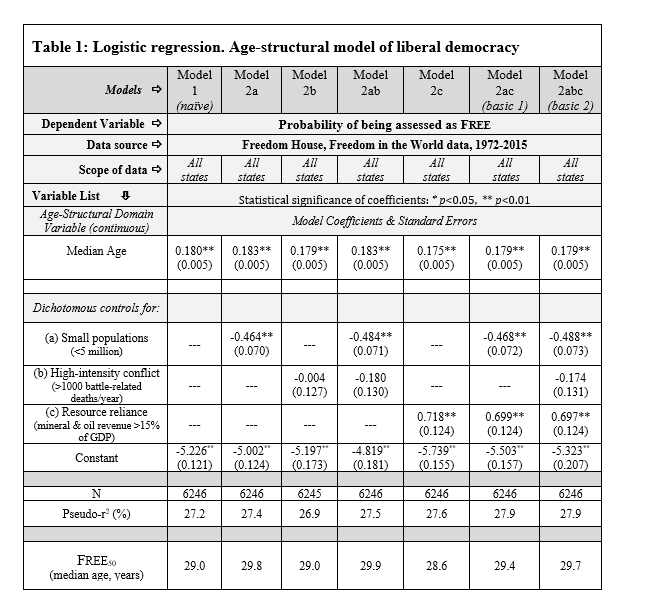
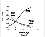
The age-structural model of liberal democracy (ASM-LD) generates timed expectations of the likelihood of being assessed at a high level of democracy across the age-structural axis (Fig. 2). The ASM-LD is the most well-studied of all age-structural functions, having been investigated by three independent research efforts, each using different measures of age structure (several variations of “youth bulge” measures, median age), and various indicators of democracy. Indications of democracy include Freedom House’s Free status (Cincotta 2008, 2008-09), high levels (8 to 10) of Polity IV regime scores (Cincotta & Doces, 2012; Weber, 2012), and high levels of voting as a proportion of eligible voters (Dyson, 2013). The conclusions were similar. Moreover, the ASM-LD is the subject of several successful forecasts and statistical experiments, which in turn have inspired additional hypotheses and modeling (Cincotta, 2008-09; Cincotta & Doces, 2012; Cincotta, 2015a, 2015b).

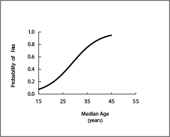
Figure 2. An example of a Class II function: the age-structural function depicting the probability of being assessed as FREE in Freedom House’s annual survey.

The functional form of the ASM-LD, shown here (Fig. 2), plots the timed expectation of attaining Free in Freedom House’s annual survey (Model 2ac, Table 1), as a probability calculated across the age-structural domain (Cincotta, 2015b). The most rapid pace of shifts to Free from lower categories should be expected to occur around the theoretical infliction point, where the probability of being assessed as Free is 0.50. This point, called Free50, is at about 29.5 (+0.5) years of median age.

A Class III Function: The Presence of Intra-state Peace.

The Age-structural Model of Intra-state Peace (ASM-ISP) predicts the probability of the absence of intra-state conflict across the age-structural domain (Fig. 3). The model draws its data on the presence or absence of intra-state conflict (>25 battle-related deaths per year) from the UCDP-PRIO Conflict Database, maintained and published cooperatively by the Uppsala Conflict Database Project (UCDP) and Peace Research Institute of Oslo (PRIO) (UCDP/PRIO, 2016; Gleiditsch et al., 2002; Themnér & Wallensteen, 2013). Its function (Fig. 3) is a class III age-structural function, based upon the ASM-ISP, with controls for small population (<5.0 million), and natural resource reliance (resource rents <15.0 percent of GDP).

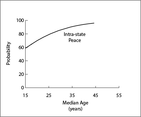
Figure 3. An example of a Class III function: the age-structural function of intra-state peace (absence of an intra-state conflict).

The ASM-ISP is neither a tightly fit nor strongly predictive model—its gradual slope is not conducive to forecasting. It is nonetheless useful in mapping states, now and over the next two decades, that are generally vulnerable to the outbreak of intra-state conflict and other forms of political violence. It is worth noting that, according to the ASM-IP, at a median age of 15.0 years, roughly 60 percent of all states are unlikely to be experiencing an intra-state conflict.  Further investigations of the function indicate that while civil conflicts appear almost exclusively in the youthful portion of the age-structural domain (median age of 25 years or less), ethnoreligious conflicts extend throughout the domain (see Yair, 2016).

Attachments

The Age-structural Transition

The Course of the Age-structural transition. 

The course of the age-structural transition is pictured by positioning the world’s states (in 2015) in terms of their proportion of young people (less than 30 years of age) and seniors (65 and older).

Initiated by fertility decline, the age-structural transition entails gradual shifts in the relative size of age cohorts through a lengthy, relatively predictable series of configurations. The Age-structural Theory of State Behavior owes much of its predictive potential to: (a.) the power of these configurations to influence, amplify, control, and reflect, a broad range of interacting demographic, social and economic conditions; and (b.) the ability of demographers to project future configurations using cohort component methodologies.

To describe the age-structural transition with some narrative clarity, I employ the classification system published in the (U.S.) National Intelligence Council’s Global Trends series of publications (National Intelligence Council [NIC], 2012, 2017). This system divides the transition into four distinct phases, based on country-level median age (the age of the “middle person”, for whom 50 percent of the population is younger): the youthful; intermediate; mature; and post-mature phases.

However, the age-structural transition is a continuous process. It is advanced by fertility decline and by higher rates of survival at old age. However, median ages can become younger as childhood mortality declines in the absence of fertility decline. The impact of migration on the age structure depends upon the age-structure of the in-migrants and out-migrants.

Getting “Unstuck” from Chronological Time

State Behavior in Age-structural Time


The most discussed breakthrough in international political theory over the past decade appears to be Nassim Taleb’s formulation of the “Black Swan hypothesis. Taleb argues that the dynamics of state behavior are so complex and hidden that political outcomes and their timing are generally impossible to forecast. Others (including myself) read Taleb’s thesis as an exhaustingly lengthy excuse–a disheartening admission that the endeavor of forecasting state political behavior is beyond the capacity of current social science. Taleb’s treatise follows on a study published by Philip Tetlock in 2005, which reported on a 15-year experiment that the author ran with the consent of a group of highly qualified political scientists. Tetlock found that when these seasoned academics chose among predicted futures based on current political theories and the full wealth of their experience, they could perform no better than the guessing average.

Table 1.  Logistic regression statistical table for the age-structural model of liberal democracy (likelihood of being assessed as FREE in Freedom House’s annual survey of civil liberties and political rights).

Whereas political analysts expect political outcomes to be generated, over time, by the activities and evolving relationships of political actors, political demographers find that most states that have populations with similar age structures (distributions of residents, by age) behave similarly. Rather than evolving over time, these state behaviors appear to be timed by the movement of country-level populations through the age-structural transition–the position and pace of which has been called “age-structural time.” Thus, political demographers tend to analyze state behaviors over the course of the age-structural domain–an X axis measured in median age (a indicator of the maturity of a country’s age structure).

Why has this form of analysis yielded new insights? Over the past two decades, economic and political demographers have proposed and tested theories that identify demographic changes as key factors in a range of economic and political transitions (reviewed by Cincotta, 2012, and by Goldstone, 2012). Whether or not these are causally related, either directly or complexly, is a contentious topic that is the subject of debate among economic demographers and economists, and political demographers and political scientists.

The list of state-level effects that are associated with fertility decline and age-structural change is surprisingly long, and the effects are politically consequential. These country-level effects include: the onset of intrastate conflict (Möller, 1968; Mesquida and Weiner, 1999; Goldstone, 2002; Urdal, 2006; Cincotta and Leahy 2007); employment (Easterlin, 1968); women’s participation in the workforce (Bauer, 2001); democratization and democratic stability (Cincotta, 2008, 2009, 2013; Weber 2012; Cincotta and Doces, 2012; Dyson, 2013); the accumulation of government and household savings (Higgins and Williamson, 1997; Lee and Mason, 2011); economic development (Williamson, 2001; Bloom et al., 2002); societal investments in education (Lee and Mason, 2011); and the accumulation of public debt (Eberstadt and Groth, 2010; Lee and Mason, 2011).

For defense and foreign policy analysts, the implications of these findings are noteworthy. They indicate that, for a number political and economic transitions, modern states appear to perform more predictably when these variables are monitored as a response to changes in the configurations of their age-structure, than they do when monitored in chronological time. Therefore, analysts should expect to improve aspects of their analyses by shifting countries onto the age-structural time domain—an X-axis measured in years of median age (the age of the “middle person,” for whom 50 percent of the population is younger, and the other 50 percent is older).

For analysts tasked with early warning, shifting to age-structural time has a substantial advantage. Because UN demographers biennially generate demographic projections (demographic scenarios of the future) for each currently extant state, the future ceases to be a barrier to analysis. In other words, age-structural models that were originally fit to historic data—observations drawn from the demographic and political outcomes of countries that have already advanced through the age-structural transition—can statistically predict future trends by using projected (future) median ages as their inputs.

Unlike conventional historians and political scientists, analysts using age-structural methods need not be “stuck” in the chronological time domain. They can move back and forth, shifting from chronological time (the year) into age-structural time (the median age), in order to make a statistical prediction. And then they can re-transform their predictions, returning to chronological time—the domain in which intelligence consumers operate—to report their timed early warnings.


Statistical Methods & Tables

Age-structural modelling


In the statistical analysis shown below (Table 1), the logistic regression model employs the country-level median age as the only continuous independent variable. In these “age-structural analyses”, logistic regression has been used to determine (1.) whether, or not, the presence of a specific, discrete condition (the dependent variable; 0 or 1) varies as states advance across the age-structural transition. If, indeed, it varies across this transition, then (2.) age-structural methods proceed to determine how that specific condition varies (its functional form); and (3.) the level of certainty that is associated with that variation (its confidence interval).

In age-structural models, the dependent variable (composed of data coded “1” or “0”) must be discrete, or discretized by creating a gradient of discrete categories. Examples of discrete conditions include the presence or absence (in a year) of a type of political regime, such as a liberal democracy (shown in Table 1), or the presence or absence of an intra-state conflict. Examples of discretized variable include the attainment of specific levels of per-capita income (e.g., the World Bank’s Upper-middle Income Category), or levels of educational attainment (secondary school participation).

Table 1.  Logistic regression statistical table for the age-structural model of liberal democracy. Dichotomous controls are small populations, the presence of high-intensity conflict, and reliance on oil or mineral resources (each defined in the table). 


Control Variables

In my own experience, I have found it useful to begin with the simplest form of the age-structural model—the naïve model, which is devoid of any control variables (Model 1, example in Table 1). To refine this model, I have added dichotomous (presence or absence) control variables, or combinations of these three variables, to refine the naïve model. States with these qualities often, but not always, perform differently than the larger group of states. Before graphing the function, running experiments with other dichotomous variables, or identifying exceptional states, I typically find it useful to control for these three factors, depending on the dependent variable:

(a.) States with small populations.  This factor identifies states with a mid-year population of fewer than 5.00 million. The source of this estimate was the UN Population Division’s 2015 revision of World Population Prospects (UNPD, 2015).

(b.) States engaged in high intensity conflict. A state is deemed to be in high intensity conflict if, for that year, it experiences more than 1000 battle-related deaths, according to the current version of the UCDP Conflict Dataset (Uppsala Conflict Data Project and Peace Research Institute, Oslo [UCDP/PRIO], 2014; Gleditsch et al., 2002).

(c.) Resource-reliant states. A state was deemed as experiencing significant oil and mineral wealth if revenues from these resources comprised over 15.0 percent of GDP. Annual levels of oil revenue, mineral revenue and GDP were obtained from the 2015 version of the World Bank’s World Development Indicators (World Bank Group [WB], 2015).

Thus, current analyses typically feature controlled models (Model 2, examples in Table 1) that feature various combinations of this model (e.g., Models 2a, 2ab, 2ac, 2bc, 2abc).  As a general observation, the effect of small population (a) generally produces the strongest statistical impact on a naïve model. The control for high intensity conflict (b) has occasionally been statistically significant, particularly in health and income-related models, but is omitted when the dependent variable is a conflict-related variable. Oil-mineral reliance (c) has been statistically significant in most age-structural models.

Attachments

Age-structural Models

Age-structural Models: the Idea


The age-structural domain is the unifying feature of Age Structural Theory. Rather than consider relationships over chronological time, age-structural models re-position state behaviors on the age-structural domain—an X-axis that follows the continuous path of the age-structural transition, situating it as the principal independent variable. The age-structural domain, measured in median age, is the only continuous independent variable in logistic regression analysis. All controls and treatment variables are dichotomous (0,1). Likewise, the functional forms that are fitted to data by logistic regression are displayed across a domain beginning at a median age of 15 years and ending at 55 years.

Each age-structural model begins as a hypothesis, whether generated notionally (from theory) or observationally, that a measurable state behavior is typically associated with the movement of states through the age-structural transition. It is important to stress—and periodically re-iterate—that these models begin as a hypothesis that is epistemologically situated at the very edge of Age-structural Theory. Some age-structural models have been strengthened and brought into the more certain body of theory by repeated in-sample testing, out-of-sample testing, and some form of successful prediction. A few others—particularly hypotheses associated with the age-structural model of liberal democracy (ASM-LD)—have demonstrated their utility by out-competing other methods of analysis and by exposing original insights into the processes under study.

In my analyses, age-structural models employ the country-level median age as the only continuous independent variable. In these analyses, logistic regression has been used to determine (1.) whether, or not, the presence of a specific, discrete condition (the dependent variable) varies as states advance across the age-structural transition. If, indeed, it varies across this transition, then (2.) age-structural methods proceed to determine how that specific condition varies (its functional form); and (3.) the level of certainty that is associated with that variation (its confidence interval).

In age-structural models, the dependent variable (composed of data coded “1” or “0”) must be discrete, or discretized by creating a gradient of discrete categories. Examples of discrete conditions include the presence or absence (in a year) of a type of political regime, or the presence or absence of an intra-state conflict. Examples of discretized variable include the attainment of specific levels of per-capita income (e.g., the World Bank’s Upper-middle Income Category), or levels of educational attainment (secondary school participation).

For logistic regression to produce a reasonable fit to these data, the frequency of the dependent variable, as it is sampled across the age-structural domain, must be adequately described by a logistic function—a monotonic sigmoid curve generated by the Verhulst equation (an S-shaped function, beginning low and approaching an upper asymptote), or to some segment of a logistic curve (Maynard, 2001). Therefore, a segment of a logistic function can neither be fit adequately to frequency data that (a.) rises substantially and then falls, nor (b.) falls substantially and then rises again across the domain.

Age-structural Theory is a reductionist project. Operating on a single, continuous X-axis simplifies statistical analyses and permits the visual display of relationships on a two-dimensional graph. And, like all simplified statistical theories, it has limitations. Firstly, it suffers from the “small number problem”—predictions are most successful when considering clusters of states, rather than betting on a single state. Secondly, by itself, taking only median age into account, age-structural models are blind to the influence of non-demographic and sub-national demographic factors. Unless these are noted through observation, studied through separate analyses, or added experimentally as discrete (0,1) variables to the statistical analysis, its reliance on the country-level scalar measure of median age as the lone continuous domain of its analysis can obscure important factors. For example, observations of the functional form of the age-structural model of liberal democracy have shown that presence of a small population size (under 5 million) and regime types have substantial impact on outcomes (Cincotta, 2015a, 2015b; Weber, 2013).

In its classic form (which was used to describe constrained population growth), the logistic function begins at its lowest point, accelerates to an inflection point, decelerates, and then levels off as it approaches an upper asymptote. However, this function can also be parameterized to operate in reverse: to begin at its high point and descend to a lower asymptote. Upward or downward sections of the function can be fit to data, as well.